All-in-one data structures and algorithms cheatsheet
September 15, 2022
⏳ 67 min read
Preface
This is my own curated list of tips and tricks about data structures and algorithms, in Python or TypeScript.
Checklist
If you are able to bring up complexities amd implementations in mind just by looking at each topic, you are in a good shape.
Big-O and its friends
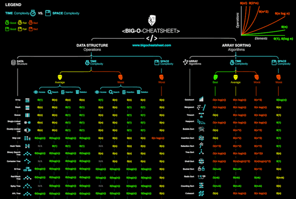
Big O cheatsheet
Everything is from bigocheatsheet.com. It’s just that I don’t visit it as often as my blog.
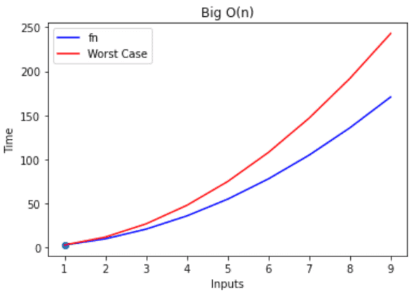
Mathematical definition of Big-O
if there exists and where for some
Intuitive definition of Big-O
- Worst time complexity of an algorithm. Denotes an upper boundary.
- How fast a program’s runtime grows asymptotically when the size of the input increases towards infinity
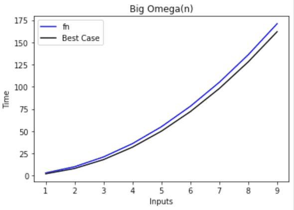
Mathematical definition of Big-Omega
if there exists and where for all
Intuitive definition of Big-Omega
Best time complexity of an algorithm. Denotes a lower boundary.
Mathematical definition of Big-Theta
In other words,
Intuitive definition of Big-Theta
It must be the case that is essentially the same function as if the constants on each function are removed, if any.
Big-O computations
- If is a sum of several terms, the term of the largest growth rate can be left without others because we only care about the biggest term}|
- example:
- If is a product of several factors, any constants C terms in the product that do not depend on can be omitted.
- example:
- Proving Big-O often requires choosing an arbitrary and :
- example: show that
- proof:
Review of exponents
Rule of power
- Rule:
- Example:
Multiplying exponents
- Rule:
- Example:
Dividing exponents
- Rule:
- Example:
Rule Taking the power of two multiplied terms
- Rule:
- Example:
Review of Logarithms
Relationship between the logarithm and the exponent function
The logarithm is the inverse of the exponent function.
example:
Log of a product
- Rule:
- Example:
- Reasoning:
Log of a fraction
- Rule:
- Example:
- Reasoning:
Log of a power
- Rule:
- Example:
- Reasoning:
A power of a log
- Rule:
- Example:
- Reason:
Change of a base
- Rule:
- Example:
Amortized analysis
Amortized analysis is a worst-case analysis of a a sequence of operations to obtain a tighter bound on the overall or average cost per operation in the sequence than is obtained by separately analyzing each operation in the sequence.
There are two prominent examples:
- Amortized of
array.append() - Amortized of
dict[key]
Arrays
- An array can work as a replacement for hash tables if you know the range of indices that will go into the array. But sometimes it will waste spaces.
- otherwise, do use hash tables because they have O(1) amortized time complexity.
append()orpush()for arrays and strings takes O(1) amortized time. It means that on average it will take O(1) for insertion if you keep adding new elements. This is because it takes O(1) time for simple insertions with no capacity increase, but it will take O(n/2) time for insertions with capacity increase, where n is the size of next array (because usually arrays double the capacity). The insertion with capacity increase only comes when you reach n/2 elements. This is why on average the insertion would take O(1) time.
Useful code snippets
Initialize an empty array of length 10 full of 0’s:
const arr = Array(100).fill(0)arr = [0] * 10Be careful when you are creating a 2D array in Python:
doesnt_work_arr = [[0] * 10] * 10 # doesn't work
2d_arr = [[0] * 10 for _ in range(10)] # works
Creating an array of certain range of contiguous characters:
count = [0] * (ord("z") - ord("a") + 1)

# access the index corresponding to "c" (should be 2nd index)
count[ord("c") - ord("a")]
Remember that uppercase letters come first in the ASCII order (and there are some special characters in between "Z" and "a")
>>> ord("A")
65
>>> ord("Z")
90
>>> ord("a")
97
>>> ord("z")
122
Why an arraylist has armortized insertion time
Basic idea
- An arraylist has:
- : the actual number of elements in the list
- : the size of the memory allocated for the list (always bigger than or equal to )
- Appending an element to an list while its length is less than or equal to the is an apparent
- When the is full, (= ) elements need to be copied over to a brand new list, which is not
The cost of resizing
- Usually, the list will need to double in its (powers of 2). Therefore, list increases its only when for some integer (you need to resize at ).
- Total number of times for resizing is . At certain , the list would have been resized for times. For example, if your is , that means is the list would have been resized for times.
- The total (accumulated) cost of resizing at :
- We know . For example,
- Therefore, the total accumulated cost of resizing at = where is the number of times of resizing.
The cost of ops
- Up to a certain , the accumulative cost of operations is . For exmaple, let . Other ops are all resizing ops at 2, 4, 8, and 16 (you don’t resize at 1).
- Because we are interested in the amortized time complexity, we will have to divide the entire cost by .
- is the general worst case, since the last operation (the part) triggers the resizing.
Conclusion
Sliding window
- Sliding window technique is used in subarray or substring problems, like longest, shortest, or target value.
- For these problems, there is usually an apparent brute force solution that runs in O(N²), O(2^N)
- Two pointers move in the same direction in the way that they will never overtake each other (O(n))
- The key concept is you want to keep track of the previous best information you have
Intuition
FYI: Big help from this stackoverflow answer.
Sliding window can be used when you want to efficiently get the maximum sum of a subarray of length 5 in an array, for example.
[ 5, 7, 1, 4, 3, 6, 2, 9, 2 ]The bruteforce algorithm will clearly introduce O(length_of_the_array * length_of_the_subarray) time complexity. But we can improve by ‘sliding the window’:
- The first subarray’s sum is sum(5, 7, 1, 4, 3) = 20
- The second subarray’s sum is sum(7, 1, 4, 3, 6) = 21
- … and so on
But the only numbers changing in the calculation are the first and the last number (5 and 6). So simply subtracting 5 from and adding 6 to the first subarray’s sum would deduce the second array’s sum. The same goes for the next subarrays.
This will result in O(n) time complexity because subtracting and adding ops are fixed at 2 * O(1) regardless of length of the array/subarray.
Sliding window of dynamic range
- Sometimes, the sliding window’s length is not fixed. In this case, you will need to move the
startandendpointers to the array dynamically. - Dynamic range sliding window qs often involes using a hash to store previous information and starting again from there once some condition is met
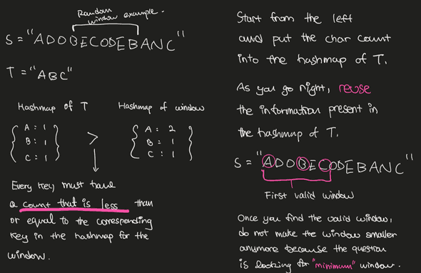
👉 Example 1: Minimum window substring
Input: s = "ADOBECODEBANC", t = "ABC"
Output: "BANC"
Explanation: The minimum window substring "BANC" includes 'A', 'B', and 'C' from string t.
from collections import defaultdict
from typing import Dict
def minimum_window_substring(s: str, substr: str) -> str:
substr_hash: Dict[str, int] = defaultdict(int)
window_hash: Dict[str, int] = defaultdict(int)
# for "ABCDAB", need_unique_chars_count will be 4 because A and B overlap
# it's just len(substr_hash)
need_unique_chars_count = 0
for c in substr:
if substr_hash[c] == 0: need_unique_chars_count += 1
substr_hash[c] += 1
have_unique_chars_count = 0
minimum_window_bounds = [-1, -1]
start = 0
# initiate 'end' from the beginning of the string
for end in range(len(s)):
if s[end] in substr_hash:
window_hash[s[end]] += 1
# minimum requiremenet to create a window
# for this char (which is s[end]) has been fulfilled
if window_hash[s[end]] == substr_hash[s[end]]:
have_unique_chars_count += 1
# while the condition to create a valid sliding window has
# been fulfilled
while have_unique_chars_count == need_unique_chars_count:
curr_window_size = end - start + 1
# current valid window size is smaller than the existing one
# therefore we need to replace the window
if minimum_window_bounds[0] == -1 or curr_window_size < minimum_window_bounds[1] - minimum_window_bounds[0] + 1:
minimum_window_bounds = [start, end]
# keep shrinking from the leftmost character because
# we checked everything with it
window_hash[s[start]] -= 1
# if you happen to take out the character
# that was required for the minimum window,
# decrement have_unique_chars_count by 1
if s[start] in substr_hash and window_hash[s[start]] < substr_hash[s[start]]:
have_unique_chars_count -= 1
start += 1
if minimum_window_bounds[0] == -1:
return ""
return s[minimum_window_bounds[0]:minimum_window_bounds[1] + 1]Complexities:
- time O(len(s) + len(substr)) because both
startandendpointer scan the stringsfor only one time. - space: O(len(s) + len(substr)) because all we use is the hashmap for each string.
👉 Example 2: Minimum Size Subarray Sum
Input: target = 7, nums = [2,3,1,2,4,3]
Output: 2
Explanation: The subarray [4,3] has the minimal length under the problem constraint.
import math
class Solution:
def minSubArrayLen(self, target: int, nums: List[int]) -> int:
if len(nums) == 0:
return 0
left = 0
subarray_sum, subarray_len = 0, math.inf
# right pointer always increases
for right, num in enumerate(nums):
subarray_sum += num
# if the subarray's sum satisfies the condition,
# increase the left pointer until the subarray's sum
# does not satisfy the condition anymore
while subarray_sum >= target:
subarray_len = min(right - left + 1, subarray_len)
subarray_sum -= nums[left]
left += 1
return 0 if subarray_len == math.inf else subarray_lenComplexities:
- time:
- space: O(1)
Index as a hash key
-
The index can be used as a hash table holding index and boolean value as key and value without forgetting about the initial value itself
Example:
arr = [4,1,5,2,2]

for n in arr:
  if n < len(arr) and n > 0 and arr[n] > 0:
    arr[n] *= -1

has_three = arr[3] < 0 # false
has_two = arr[2] < 0 # true
Two pointers
Quite similar concept to the sliding window. Need to use two pointers each pointing at different parts of the array.
Traversing from the right
Sometimes you need to start from the back of the array.
Sorting the array
- If an array is sorted, there may be more optimal solution
- Sorting an array may simplify the problem
Precomputation
Precomutation of prefix/suffix/sum/product might be useful
Strings
- Watch out for the range of the input strings (characters): for example,
atoz.
Hash table (Hash map)
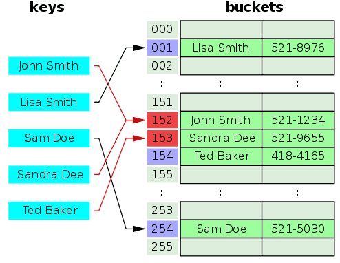
A hash table stores data in a key-value pair. In a ‘good’ implementation of a hash table, the lookup by key takes amortized time which can be mathematically proven.
Hash table implementation logics
- An array is a random access data structure, meaning that any index can be accessed in time.
- A hash table is an abstract data structure because the underlying data structure can usually be an array. It does something called hashing, which is a translation from an arbitrary key to an integer number that behaves as an index of an array.
- The length of the array can be much smaller than the number hashcodes (output of the hash functions).
- For that reason, two different hashcodes may end up in the same array index. This is called collision.
- In a terrible hash table with bad a hash function that causes lots of collisions, the lookup may take .
Hash function
A hash function used for a hash table, where is an integer key, is the maximum positive integer key, and is some integer that is , can be defined as follows:
If , is not injective (one-to-one) by pigeonhole principle. In other words, . This is called collision. A method to handle this will be soon introduced.
A simple hash function can be implemented by getting a remainder which is k % m in Python, where is an appropriate prime number:
For example,
This function works the best only when keys are uniformly distributed. For example, let’s say you got . And what if you put the elements of the set into the hash table? The remainder will always be 1, and the lookup time will take .
Therefore, we want the performance of our data structure to be independent of the keys we choose to store.
Universal hashing
For a large enough key domain , every hash function will be bad for some set of inputs. However, we can achieve good expected bounds on hash table performance by choosing our hash function randomly from a large family of hash functions.
The definition of the set of hash functions we are looking for is as follows:
Let be the set of universe keys and be a finite collection of hash functions mapping into . Then is called universal if,
In plain terms, for all that belong to and are distinct from each other, the cardinality of pairs of that collide with each other (where belongs to ) is equal to the cardinality of the set of hash functions divided by .
To put it even easier: the probability of a collision for two different keys and given a hash function randomly chosen from is . This is can easily be seen because
Collision resolution strategies
As discussed, a collision must happen anyway when there are slots and items to insert into the slots, where , due to the pigeonhole principle. Here are the strategies to resolve the collision.
1. Separate chaining.
- Easiest technique to resolve this problem.
- Whenever there is a collision, append the new data to a linked list (called a bucket) allocated to that specific index of the array.
- A node in the linked list would contain the original key and value.
- The hashcode will be used to iterate through a linked list that corresponds to the key.
The structure may be better described with TypeScript:
interface KeyValNode<T> {
  key: number; // hashcode
  val: T; // data to be held
  next: KeyValNode<T> | null;
  prev: KeyValNode<T> | null;
}

type HashTable<T> = LinkedList<KeyValNode<T>>[];
2. Linear probing.
- one method of open addressing
- No linked list, directly store data in the array records
- used when there are more slots in the array than the values to be stored
- If there is a collision, store the data at
(index + n) % hash_table_lenwherenis the firstnth index at which you find the array slot is empty. For example, if you wanted to insert data at index 5 but notice it’s not empty but index 6 is, simply put it at 6. - Formally, the linear probing function can be given by where
- Usually, would just be in its simplest form.
- is the length of the array
3. Quadratic probing.
- another method of open addressing
- similar to linear probing, but the interval between probes increases quadratically. Resolve collisions by examining certain cells (1,4,9, …) away from the original probe point
- therefore, it does not check all slots in the array and may not find a vacant slot in the end
- clustering
- quadratic probing function: , where
- is the original hash function (probably just )
- is the hash function for each index
- is the length of the array
4. Double hashing.
- another method of open addressing
- double hashing function: where and are two ordinary hash functions.
- For a popular case, let and
- Let a well chosen prime number less than , and be the length of the array
- For a popular case, let and
Importance of the load factor
- As load factor increases towards 100%, it becomes increasingly difficult to find/insert a given key.
- That is why the load factor is normally limited to 70~80% at maximum and for some algorithms just 50%.
- Once the load factor exceeds the boundary, double the array size, and rehash every element again
Collision resolution strategies comparision
Strategy Separate Chaining Linear probing Quadratic probing Double hashing
Amortized analysis
👉 Hash table implementation
👉 Useful references
- http://www.mi.fu-berlin.de/wiki/pub/Main/GunnarKlauP1winter0708/discMath_klau_hash_II.pdf
- https://www.cs.bu.edu/faculty/homer/537/talks/SarahAdelBargal_UniversalHashingnotes.pdf
- https://ocw.mit.edu/courses/6-006-introduction-to-algorithms-spring-2020/ce9e94705b914598ce78a00a70a1f734_MIT6_006S20_lec4.pdf
- https://www.cs.jhu.edu/~langmea/resources/lecture_notes/130_universal_hashing_pub.pdf
- https://courses.cs.washington.edu/courses/cse525/13sp/scribe/lec5.pdf
- https://cs.stackexchange.com/questions/249/when-is-hash-table-lookup-o1
Hash table tips in Python
Use defaultdict in Python instead of checking for the key every time:
from collections import defaultdict

somedict = {}
print(somedict['test1']) # KeyError
# check if key exists
print('test1' in somedict)

somedict2 = defaultdict(int)
print(somedict2['test2']) # 0

# custom initialization
somedict3 = defaultdict(lambda: 3)
print(somedict3['test3']) # 3
Stack
You can easily simulate the behavior of a stack using a list in Python or array in JavaScript.
👉 Stack implementation
from typing import TypeVar, Generic, Union

T = TypeVar('T')

class Stack(Generic[T]):
  def __init__(self):
    self.arr = []

  def __len__(self):
    return len(self.arr)

  def pop(self) -> Union[T, None]:
    return self.arr.pop()

  def push(self, item: T) -> None:
    self.arr.append(item)

  def peek(self) -> T:
    if len(self.arr) == 0:
      raise Exception("Length is zero")

    return self.arr[-1]
Queue
Standard queue
A normal queue would work in a FIFO fashion. In most cases, you would use Python because it has a queue built into its stdlib.
| op | explanation | time complexity |
|---|---|---|
| put | inserts an item into the back of the queue (also called ‘enqueue’ or ‘prepend’). | O(1) |
| get | removes and returns an item from the front of the queue (also called ‘dequeue’ or ‘pop’). | O(1) |
| .queue | returns a data structure that can be referenced just like a list | - |
👉 Standard queue implementation
from typing import Generic, TypeVar
from doubly_linked_list import DoublyLinkedList

T = TypeVar("T")

class Queue(Generic[T]):
  def __init__(self):
    self.dll = DoublyLinkedList()

  def is_empty(self):
    return len(self.dll) == 0

  def prepend(self, value: T):
    self.dll.insert_at(0, value)

  def pop(self) -> T:
    return self.dll.remove_at(len(self.dll) - 1)

q = Queue[int]()

print(q.is_empty())
q.prepend(1)
print(q.pop()) # 1
q.prepend(2) # 2 1
q.prepend(3) # 3 2 1
print(q.pop())
q.prepend(4) # 4 3 2 1
print(q.is_empty()) # false
print(q.pop()) # 1
print(q.pop()) # 2
print(q.is_empty())
Deque
A queue with two ends.
| op | explanation | time complexity |
|---|---|---|
| appendleft | appends an item to the left of the queue | O(1) |
| popleft | removes and returns an item from the left of the queue | O(1) |
| append | appends an item to the right of the queue | O(1) |
| pop | removes and returns an item from the right of the queue | O(1) |
[index] |
references the index of a deque just like a list | O(1) |
👉 Deque implementation
from typing import Generic, TypeVar
from doubly_linked_list import DoublyLinkedList, debug

T = TypeVar("T")

class Deque(Generic[T]):
  def __init__(self):
    self.dll = DoublyLinkedList()

  def is_empty(self):
    return len(self.dll) == 0

  def append(self, value: T):
    self.dll.insert_at(len(self.dll), value)

  def prepend(self, value: T):
    self.dll.insert_at(0, value)

  def pop(self) -> T:
    return self.dll.remove_at(len(self.dll) - 1)

  def popleft(self) -> T:
    return self.dll.remove_at(0)

q = Deque[int]()

deque = Deque()

deque.prepend(1)
deque.prepend(2)
deque.prepend(3)
deque.prepend(4)
debug(deque.dll) # 1

deque.append(5)
deque.append(6)
debug(deque.dll) # [4,3,2,1,5,6]

deque.popleft() # 4
deque.pop() # 6
debug(deque.dll) # [3,2,1,5]
Priority queue
- All elements in a priority queue need to have a priority associated with them.
- The queue will maintain a sorted order throughout its lifetime
- uses
heapq(heap data structure) internally
| stdlib op | explanation | time complexity |
|---|---|---|
| put | inserts an item into the queue (also called ‘enqueue’). | |
| get | removes and returns an item from the queue (also called ‘dequeue’). | |
| .queue | returns a data structure that can be referenced just like a list | - |
from queue import PriorityQueue

q = PriorityQueue()

q.put((2, 'code'))
q.put((1, 'eat'))
q.put((3, 'sleep'))

q.queue # [(1, 'eat'), (2, 'code'), (3, 'sleep')]
while not q.empty():
    next_item = q.get()
    print(next_item)

#   (1, 'eat')
#   (2, 'code')
#   (3, 'sleep')
👉 Priority queue implementation using heapq
from typing import Generic, Tuple, TypeVar, Union
import heapq

T = TypeVar('T')

class PriorityQueue(Generic[T]):
  def __init__(self):
    self.heap = []

  def put(self, item: T):
    heapq.heappush(self.heap, item)

  def get(self) -> Union[T, None]:
    if not self.heap:
      raise Exception("No elements in the heap")

    return heapq.heappop(self.heap)

  def __len__(self) -> None:
    return len(self.heap)

  def __bool__(self) -> bool:
    return len(self.heap) != 0
pq = PriorityQueue[Tuple[int, str]]()

pq.put((1, "one"))
pq.put((5, "five"))
pq.put((2, "two"))
pq.put((10, "ten"))

while pq:
  # (1, 'one')
  # (2, 'two')
  # (5, 'five')
  # (10, 'ten')
  print(pq.get())
Linked lists
Singly linked list implementation
👉 Singly linked list implementation
from typing import Iterator, Union


class Node:
  def __init__(self, value=None, nxt=None, prev=None):
    self.value = value
    self.nxt = nxt
    self.prev = prev

  def __str__(self) -> str:
    return f"{{value:{self.value}}}"

class SinglyLinkedList:
  def __init__(self):
    self.head = Node()
    self.len = 0

  def __len__(self):
    return self.len

  def is_empty(self) -> bool:
    return len(self) == 0

  def connect_in_between(self, prev: Node, middle: Node, nxt: Node):
    prev.nxt = middle
    middle.nxt = nxt

  def traverse(self) -> Iterator[Node]:
    # head is a dummy pointer
    ptr = self.head.nxt

    while ptr is not None:
      yield ptr
      ptr = ptr.nxt

  def traverse_right_before(self, index: int) -> Node:
    ptr = self.head

    visit_count = index
    while ptr.nxt is not None and visit_count > 0:
      ptr = ptr.nxt
      visit_count -= 1

    if visit_count != 0:
      raise Exception(f"Index out of bounds: {index}")

    return ptr

  def insert_at(self, index: int, value) -> Node:
    prev = self.traverse_right_before(index)
    middle = Node(value)
    nxt = prev.nxt
    self.connect_in_between(prev, middle, nxt)

    self.len += 1

    return middle

  def remove_at(self, index: int) -> Node:
    prev = self.traverse_right_before(index)
    prev_nxt = prev.nxt
    two_nodes_away_node: Union[Node, None] = prev.nxt.nxt
    prev.nxt = two_nodes_away_node

    self.len -= 1
    # assert self.len >= 0

    return prev_nxt

ll = SinglyLinkedList()
def debug():
  for node in ll.traverse():
    print(node, end=" ")
  print("")

ll.insert_at(0, 1)
ll.insert_at(0, 2)
ll.insert_at(0, 3)
ll.insert_at(0, 4)
ll.insert_at(0, 5)
ll.insert_at(0, 6)
ll.insert_at(0, 1)
ll.insert_at(0, 3)
ll.insert_at(5, 100)
debug()
# {value:3} {value:1} {value:6} {value:5} {value:4} {value:100} {value:3} {value:2} {value:1}
ll.remove_at(5)
debug()
# {value:3} {value:1} {value:6} {value:5} {value:4} {value:3} {value:2} {value:1}
ll.remove_at(0)
ll.remove_at(0)
ll.remove_at(3)
debug()
# {value:6} {value:5} {value:4} {value:2} {value:1}
ll.remove_at(0)
ll.remove_at(len(ll) - 1)
debug()
# {value:5} {value:4} {value:2}
ll.insert_at(2, 50)
debug()
# {value:5} {value:4} {value:50} {value:2}
Doubly linked list implementation
👉 Doubly linked list implementation
from typing import Iterator, Union


class Node:
  def __init__(self, value=None, nxt=None, prev=None):
    self.value = value
    self.nxt = nxt
    self.prev = prev

  def __str__(self) -> str:
    return f"{{value:{self.value}}}"

class DoublyLinkedList:
  def __init__(self):
    self.head = Node()
    self.tail = Node()
    self.head.nxt = self.tail
    self.tail.prev = self.head
    self.length = 0

  def __len__(self) -> int:
    return self.length

  def traverse(self) -> Iterator[Node]:
    ptr = self.head
    while ptr:
      if ptr == self.head or ptr == self.tail:
        ptr = ptr.nxt
      else:
        yield ptr
        ptr = ptr.nxt

  def traverse_from_right(self) -> Iterator[Node]:
    ptr = self.tail
    while ptr:
      if ptr == self.head or ptr == self.tail:
        ptr = ptr.prev
      else:
        yield ptr
        ptr = ptr.prev

  def connect_in_between(self, prev: Node, middle: Node, nxt: Node):
    prev.nxt = middle
    middle.prev = prev

    middle.nxt = nxt
    nxt.prev = middle

  def traverse_up_to(self, index: int):
    if len(self) < index:
      raise Exception(f"Index out of bounds at {index}")

    ptr = self.head

    visit_count = index

    while ptr.nxt is not None and visit_count > 0:
      ptr = ptr.nxt
      visit_count -= 1

    # should never get here, but just an exhaustive check
    if visit_count != 0:
      raise Exception(f"Index out of bounds at {index}")

    return ptr

  def insert_at(self, index: int, value):
    prev = self.traverse_up_to(index)

    nxt = prev.nxt
    middle = Node(value)
    self.connect_in_between(prev, middle, nxt)
    self.length += 1

  def at(self, index: int) -> Union[Node, None]:
    if len(self) <= index:
      raise Exception(f"Index out of bounds at {index}")

    prev = self.traverse_up_to(index)
    if prev.nxt == self.tail:
      return None
    return prev.nxt

  def remove_at(self, index: int):
    prev = self.traverse_up_to(index)
    two_nodes_away_node = prev.nxt.nxt

    prev.nxt = two_nodes_away_node
    two_nodes_away_node.prev = prev
    self.length -= 1

def debug(dll: DoublyLinkedList):
  for node in dll.traverse():
    print(node, end="")
  print("")
  for node in dll.traverse_from_right():
    print(node, end="")
  print("")

doubly_linked_list = DoublyLinkedList()
doubly_linked_list.insert_at(0, 0)
doubly_linked_list.insert_at(0, 1)
doubly_linked_list.insert_at(0, 2)
doubly_linked_list.insert_at(0, 3)
doubly_linked_list.insert_at(4, 100)
debug(doubly_linked_list)
doubly_linked_list.remove_at(0)
doubly_linked_list.remove_at(3)
doubly_linked_list.remove_at(1)
debug(doubly_linked_list)
The ‘dummy head’ technique
pointing to the actual head is useful for languages where there is a no explicit expression of a pointer (like LinkedListNode *node in C++). So it would go like this in TS:
const dummyHead: LinkedListNode = new LinkedListNode()

dummyhead.next = actualHead
Singly linked list does a lot
You can do a lot without making a singly linked list a doubly linked list.
The runner technique
it employs two pointers at the same time. For example, when you want to get the middle node of the array, you can use this.
def middleNode(self, head: Optional[ListNode]) -> Optional[ListNode]:
  slow = head
  fast = head
  while fast and fast.next:
      slow = slow.next
      fast = fast.next.next

  return slow
function middleNode(head: ListNode | null): ListNode | null {
let slow = head
let fast = head
while (fast && fast.next) {
fast = fast.next.next
slow = slow!.next!
}
return slow
};Reversing the list
function reverseList(head: ListNode | null): ListNode | null {
  let curr = head
  let prev = null
  let next = null

  while (curr) {
    next = curr.next
    curr.next = prev
    prev = curr
    curr = next
  }

  return prev
}
Reversing the list may be the alternative for a variable to store values sometimes.
Cycle detection
A variation of the runner technique. Think about it this way: there are two runners in a circular track, one at a slower speed than the other. Their speeds are fixed. Then the faster one will catch up with the slower one at least once in a while. In that sense, this technique is also called tortoise and hare algorithm.
function hasCycle(head: ListNode | null): boolean {
  let slow = head
  let fast = head

  while (fast && fast.next) {
    slow = slow?.next ?? null
    fast = fast?.next?.next ?? null

    if (slow === fast) {
      return true
    }
  }

  return false
};
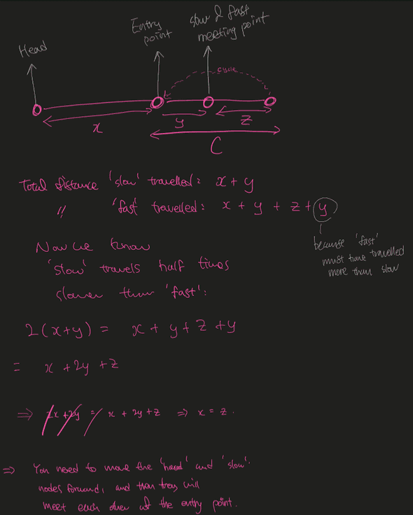
Detecting the entry node to the cycle is an extension of the code above. This however requires some mathmatical reasoning:
The crux of it is the last sentence:
You need to move the
headandslownodes forward (by one node each time), and then they will meet each other at the entry point.
function detectCycle(head: ListNode | null): ListNode | null {
  let maybeNodeInLoop = hasCycle(head)

  if (!maybeNodeInLoop) return null

  while (maybeNodeInLoop != head) {
    // practically, it never becomes null because there is a cycle
    maybeNodeInLoop = maybeNodeInLoop?.next ?? null;
    head = head?.next ?? null;
  }
  return head;
};
Trees
- A tree is an undirected and connected acyclic graph
- A tree has nodes and edges
- A tree is a recurisve data structure with subtrees
Terms
- Neighbor: Parent or child of a node
- Ancestor: A node reachable by traversing its parent chain
- Descendant: A node in the node’s subtree
- Degree: Number of children of a node
- Degree of a tree: Maximum degree of nodes in the tree
- Distance: Number of edges along the shortest path between two nodes
- Level/Depth: Number of edges along the unique path between a node and the root node
- Height of a node: Number of edges from the node to the deepest leaf
- Height of a tree: a height of the root
- Width: Number of nodes in a level
- Leaf: A node that does not have a child node in the tree
- Sibiling: nodes that share the same parent
- Subtree: basically subgraph
Binary tree
- A binary tree is a tree
- where a parent node has two edges at max, each connecting to each of two nodes.
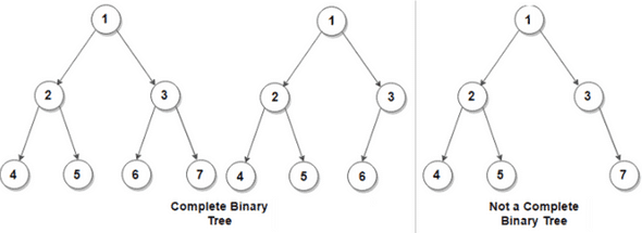
- A complete binary tree is a tree where every level of the tree is fully filled with the possible exception of the last level where the nodes must be as far left as possible. This is also a property of heap.
- A balanced binary tree is a binary tree structure in which the left and right subtrees of every node differ in height by no more than 1.
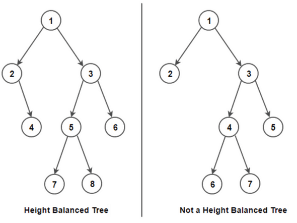
- A full binary tree is a binary tree in which each node has exactly zero or two children.

Binary search and binary search tree (BST)
A binary search is:
- an algorithm searches through a sorted collection by dividing the search set into two and comparing an element to the one that is larger or smaller than the element being searched for.
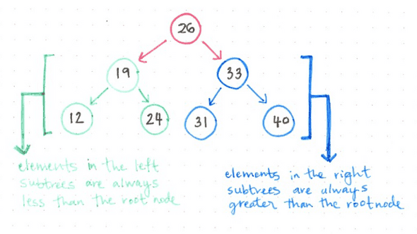
A binary search tree (BST) is a tree:
👉 General idea of binary search implementation
This post on leetcode discussion just needs pretty much everything we need in terms of binary search: Check it out.
A very general form of binary search function would look like this:
def binary_search(array) -> int:
    def condition(value) -> bool:
        pass

    left, right = min(search_space), max(search_space) # could be [0, n], [1, n] etc. Depends on problem
    while left < right:
        mid = left + (right - left) // 2
        if condition(mid):
            right = mid
        else:
            left = mid + 1
    return left
👉 General array binary search implementation
From the previous code, we can easily derive a way to implement binary search for an array.
def binary_search(nums: List[int], target: int) -> int:
    left, right = 0, len(nums) - 1
    while left < right:
        mid = left + (right - left) // 2
        if nums[mid] >= target:
            right = mid
        else:
            left = mid + 1
    return left if nums[left] == target else -1
👉 Recursive binary tree DFS from the root
def binary_tree_traversal(root: Union[Node, None]):
  if root is None:
    return
  # --
  # do what you want to do here
  # (code)
  # --
  binary_tree_traversal(root.left)
  binary_tree_traversal(root.right)
👉 Iterative binary tree DFS from the root
def binary_tree_traversal_iterative_dfs(root: Union[Node, None]):
  stack = [root]

  while stack:
    node = stack.pop()
    # --
    # do what you want to do here
    # (code)
    # --
    if node:
      stack.append(node.left)
      stack.append(node.right)
👉 Iterative binary tree BFS from the root
from queue import Queue

def binary_tree_traversal_iterative_dfs(root: Union[Node, None]):
  queue = Queue[Node]()
  queue.put(root)
  while not queue.empty():
    node = queue.get()
    # --
    # do what you want to do here
    # (code)
    # --
    if node:
      queue.put(node.left)
      queue.put(node.right)
Heap
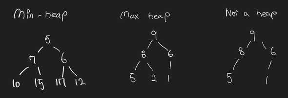
- A min heap is a complete binary tree where the smallest value is at the top.
- A max heap is a complete binary tree where the max value is at the top. (otherwise, you could negate the key of a node in a min heap to use it as a max heap)
- A binary heap usually means min heap.
- In a min heap, every node is smaller than or equal to its children (the reverse for the max heap)
- A simple rule to remember the heap ‘order’ goes left to right, top to bottom
- Questions dealing with min/max may be relevant to heap
Min heap time complexities
| Op | how | TC | TC remarks |
|---|---|---|---|
| peek (get min) | |||
| remove min | Keep swapping the value with the smallest child if the smallest child is less than the value we are bubbling down. | bubbling down would take at most time, where is the height of the complete binary tree | |
| insert a new element | Keep bubbling up while there is a parent to compare against and that parent is greater than the item | bubbling up would take at most time, where is the height of the complete binary tree | |
| overall space complexity |
Min heap implementation
👉 Min heap implementation
from typing import Generic, List, TypeVar

T = TypeVar('T')

class MinHeap(Generic[T]):
  def parent_index(self, index: int) -> int:
    return (index - 1) // 2

  def left_child_index(self, index: int) -> int:
    return index * 2 + 1

  def right_child_index(self, index: int) -> int:
    return index * 2 + 2

  def is_index_valid(self, index: int, arr: List[T]) -> bool:
    return 0 <= index <= len(arr) - 1

  def bubble_down(self, parent_index: int, arr: List[T]) -> None:
    """
    Bubble the element down until the a node is smaller than its children
    """
    while self.is_index_valid(parent_index, arr):
      left = self.left_child_index(parent_index)
      right = self.right_child_index(parent_index)

      # find the smaller one between left and right (it may not exist)
      smaller_child_index = None
      if self.is_index_valid(left, arr) and arr[left] < arr[parent_index]:
        smaller_child_index = left
      if self.is_index_valid(right, arr) and arr[right] < arr[parent_index] and arr[right] <= arr[left]:
        smaller_child_index = right

      if smaller_child_index is not None:
        arr[smaller_child_index], arr[parent_index] = arr[parent_index], arr[smaller_child_index]
        # keep bubbling down
        parent_index = smaller_child_index
      else:
        break

  def bubble_up(self, child_index: int, arr: List[T]) -> None:
      """
      Bubble the node up until the node has all of its children bigger than itself
      """
      while self.is_index_valid(child_index, arr):
        parent_index = self.parent_index(child_index)
        # if child_index == 0
        if not self.is_index_valid(parent_index, arr):
          break
        if arr[child_index] < arr[parent_index]:
          arr[child_index], arr[parent_index] = arr[parent_index], arr[child_index]
          child_index = parent_index
        else:
          break

  def peek(self, arr: List[T]) -> T:
    return arr[0]

  def push(self, arr: List[T], new_elem: T) -> List[T]:
    """
    1. Add the node to the last indexing order of the array (rightmost, bottommost part of the tree)
    2. Bubble that node up
    """
    arr.append(new_elem)
    self.bubble_up(len(arr) - 1, arr)

    return arr

  def pop(self, arr: List[T]) -> T:
    """
    1. Remove the smallest node
    2. Move the last node in the array indexing order to the first index (to the root of the tree)
    3. Bubble that node down
    """
    smallest = arr[0]
    last = arr.pop()
    if last is not smallest:
      arr[0] = last
      self.bubble_down(0, arr)

    return smallest

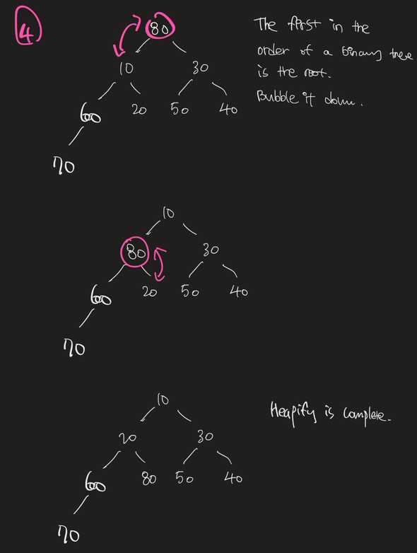
  def heapify(self, arr: List[T]) -> None:
    # last level leaves don't need to be bubbled down
    for i in range(len(arr) // 2, -1, -1):
      self.bubble_down(i, arr)
Min heap implementation logics
An array can represent a heap
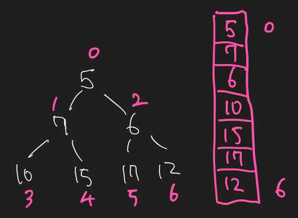
- Due to the ordering of the complete binary tree, an array can be used to represent a heap:
-
Because of the complete binary tree’s property, the indices of a parent, left child, and right child can be identified given an index:
...

def get_parent_idx(self, idx):
    return (idx - 1) // 2

def get_left_child_idx(self, idx):
    return idx * 2 + 1

def get_right_child_idx(self, idx):
    return idx * 2 + 2

...
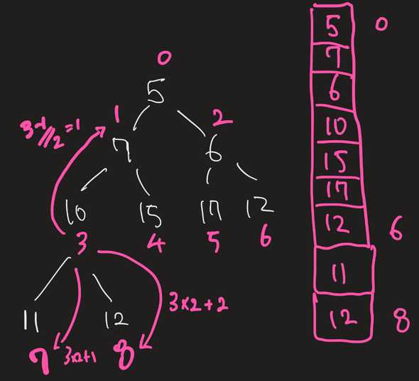
Notice the meaning of and . This is because the next level must have twice as many elements as the previous level in a complete binary tree.
For example, given an index of
3:- its parent is
3 - 1 // 2 = 2 - its left child is
3 * 2 + 1 = 7 - its right child is
3 * 2 + 2 = 8
- its parent is
Insertion
- Put the new element into the last position of the complete binary tree
- Compare the new element with its parent, and swap with the parent if it is greater than the element.
- Repeat 1-2. This process is called ‘bubbling up’
Removal
- Removal only happens at the top of the heap only
- Move the element at the last position (bottommost & rightmost) of the complete binary tree to its top
- See if any of its children are smaller than the element
- Swap the element with the smaller one of the children nodes
- Repeat 3-4. This process is called ‘bubbling down’ (also known as ‘sift down’)
Heapify: How is it ?
| Option | TC |
|---|---|
| naive approach: create an empty heap, and add the items one by one, bubbling up for times | |
| efficient approach: start from the leaf nodes at the bottom. go up each level to swap the parent with the children if it needs to be. repeat until you reach the top. |
- We all know about the naive approach by now
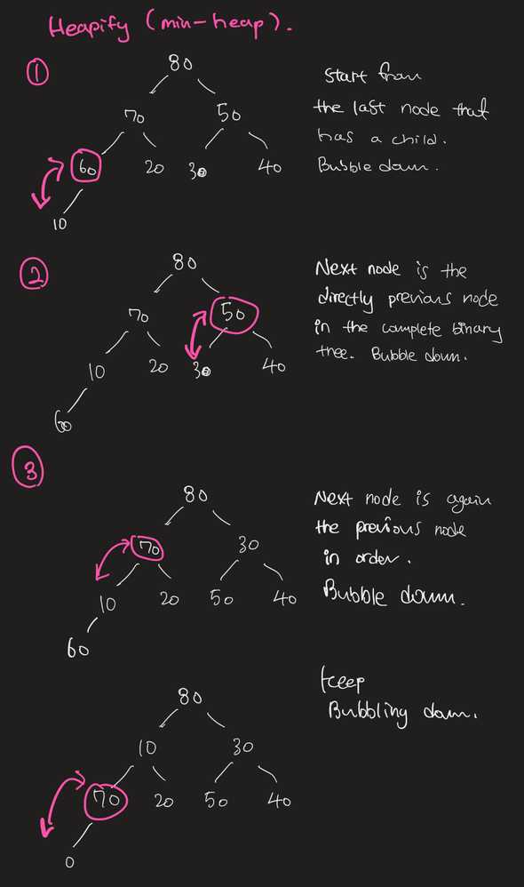
- In the efficient approach:
- start from the bottommost, rightmost node in the complete binary tree that has a child
- bubble the node down if possible
- repeat by going backwards in the array index order until the root is reached
- Why is bubbling down is much more efficient than bubbling up (FYI if implemented correctly,
bubble_upwill only need to be used to perform an insert to an existing heap)?- The number of operations required for
bubble_downandbubble_upis proportional to the distance the node may have to move. - For
bubble_down, it is the distance to the bottom of the tree, sobubble_downis expensive for nodes at the top of the tree. - With
bubble_up, the work is proportional to the distance to the top of the tree, sobubble_upis expensive for nodes at the bottom of the tree. - The tree has smaller number of nodes at the top, and larger at the bottom
- Intuitively,
bubble_downwill cost less work if every node were to be gone through
- The number of operations required for
Calculation of the work: bubble_down
As you can see, the total work for bubble_down is
where . Remember each work is the number of edges a node may have to go down at most in a single bubble_down operation.
The sum of the work is equal to . The proof requires the knowledge of some math concepts, so it’ll be skipped here.
Calculation of the work: bubble_up
The total work for bubble_up is
The first term, , is already , so it’s obvious it requires more work than bubble_down strategy.
Python’s heapq
| Description | TC | TC Description | |
|---|---|---|---|
heapq.heappush(heap: List, item: T) |
Inserts a new item and bubbles it up to fulfill heap properties | bubble_up takes time |
|
heapqq.heappop(heap: List) -> T |
Removes the smallest item in the heap and bubbles the largest element from the root down to the bottom to fulfill heap properties | bubble_down takes time |
|
heapq.heappushpop(heap: List, new_item: T) |
Inserts an item to and and then removes another from a heap. Slightly faster than separate calls to push and pop. Still the same TC | ||
heaq.heapreplace(heap: List, item: T) |
Removes an item from and then inserts an item to a heap. Slightly faster than separate calls to push and pop. Still the same TC | ||
heapq.merge(iterables: Iterable[Iterable], key: Callable, reverse: bool) |
Merge multiple sorted inputs into a single sorted output (for example, merge timestamped entries from multiple log files). Returns an iterator over the sorted values. | ?? | |
heapq.heapify(heap: List) |
Makes an array into the one that satisfies heap properties | Running bubble_down from the bottom of the tree leads to linear TC |
|
heapq.nlarest(k: int, iterable: Iterable, key: Callable) |
Get k largest elements from the collection. Note that the iterable doesn’t have to be in a ‘heapified’ state | where k is the # elements to be returned | Explained below |
heapq.nsmallest(k: int, iterable: Iterable, key: Callable) |
Get k smallest elements from the collection. Note that the iterable doesn’t have to be in a ‘heapified’ state | where k is the # elements to be returned | 1. Calls heapify on the first elements in the array. A little heap of size is created: 2. All other elements are added to the little heap using heapreplace: 3. Once step 2 is done, heappop all items from the heap and put them in an array in a reversed order: 4. Since , we can say step 2 is . 5. |
Applications of the heap
- When you feel like you can use a heap but can’t get any further, maybe think about using multiple heaps?
AVL tree
AVL trees
Red-black tree
Red-black trees
Trie (Prefix tree)
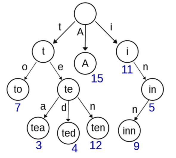
Trie is a special arrangement of nodes such that a prefix of each string is recursively stored up to the root node.
Complexities (where k is the length of a string and n is the number of strings stored)
- time
- search: O(k)
- insert: O(k)
- space: O(n * k)
A trie is useful when you need to search for matching prefix from many strings. No major languages offer this data structure in their std. Your own implementation is needed.
Note that TrieNode itself does not contain the character although from illustration of the tries above it may look like that.
👉 Trie implementation
class TrieNode:
    def __init__(self) -> None:
        # you can change this to self.nodes: List[TrieNode] = [None] * characters_len
        # if you know the exact set of characters you will receive
        self.nodes: dict[str, TrieNode] = {}
        # is_leaf tells if the node is the end of a word
        self.is_leaf = False

    def insert_many(self, words: list[str]) -> None:
        for word in words:
            self.insert(word)

    def insert(self, word: str) -> None:
        """
        recursively insert char by char
        """
        curr = self
        for char in word:
            if char not in curr.nodes:
                curr.nodes[char] = TrieNode()
            curr = curr.nodes[char]
        curr.is_leaf = True

    def find(self, word: str) -> bool:
        """
        recurisvely find char by char
        if one char in the middle is not in the tree,
        return false
        """
        curr = self
        for char in word:
            if char not in curr.nodes:
                return False
            curr = curr.nodes[char]
        return curr.is_leaf

    def delete(self, word: str) -> None:
        """
        Deletes a word in a Trie
        :param word: word to delete
        :return: None
        """

        def _delete(curr: TrieNode, word: str, index: int) -> bool:
            if index == len(word):
                # If word does not exist
                if not curr.is_leaf:
                    return False
                curr.is_leaf = False
                return len(curr.nodes) == 0
            char = word[index]
            char_node = curr.nodes.get(char)
            # If char not in current trie node
            if not char_node:
                return False
            # Flag to check if node can be deleted
            delete_curr = _delete(char_node, word, index + 1)
            if delete_curr:
                del curr.nodes[char]
                return len(curr.nodes) == 0
            return delete_curr

        _delete(self, word, 0)

def test_trie() -> bool:
    words = "banana bananas bandana band apple all beast".split()
    root = TrieNode()
    root.insert_many(words)
    # print_words(root, "")
    assert all(root.find(word) for word in words)
    assert root.find("banana")
    assert not root.find("bandanas")
    assert not root.find("apps")
    assert root.find("apple")
    assert root.find("all")
    root.delete("all")
    assert not root.find("all")
    root.delete("banana")
    assert not root.find("banana")
    assert root.find("bananas")
    return True
Graphs
DFS and BFS
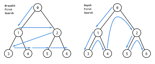
DFS: Makes a discovery into the last found vertex (branch) first.
A DFS would usually involve passing graph and visited as a reference to the function:
def dfsWrapper(edges: List[List[int]], source: int):
  graph = defaultdict(list)
  for edge in edges:
    graph[edge[0]].append(edge[1])
    graph[edge[1]].append(edge[0])
  visited = set()
  dfs(graph, visited, source)

def dfs(graph: Dict[int, List[int]], visited: Set[int], source: int):
  visited.add(source)

  for neighbor in graph[source]:
    if not neighbor in visited:
      dfs(graph, visited, neighbor)
A DFS could also be achieved using a stack, without a recursion:
def dfs(self, graph: List[List[int]]):
    stack = [0]
    seen = set(stack)
    while stack:
        i = stack.pop()
        for j in graph[i]:
            if j not in seen:
                stack.append(j)
seen.add(j)BFS: Makes a discovery into the neighbors of a vertex first before going into any other vertices.
A BFS would normally use a queue or deque which is not included in JavaScript’s native API, so other languages like Python needs to be used. This is the normal BFS with an adjacency list (edges) as an input.
from collections import defaultdict
from queue import Queue
from typing import List

def BFS(edges: List[List[int]], source: int) -> bool:
  graph = defaultdict(list)

  # O(2E) time
  for edge in edges:
    graph[edge[0]].append(edge[1])
    graph[edge[1]].append(edge[0])

  visited = defaultdict(bool)
  queue = Queue()
  queue.put(source)
  visited[source] = True
  # O(V) time
  while not queue.empty():
    vertex: int = queue.get()
    for v in graph[vertex]:
      if not visited[v]:
        visited[v] = True
        queue.put(v)
As you can see, a BFS has an O(2E + V) time complexity, which is essentially O(E + V). BFS may be more useful than DFS in general if you are looking for the shortest path.
Dealing with the adjacency list
To turn it into a graph, you may want to use not only dict but also array as long as the vertices are labeled from 0 to n:
def create_graph(edges: List[List[int]]):
  graph = [[] for _ in range(len(edges))]
  for e in edges:
    # undirected graph stored in an array
    graph[e[0]].append(e[1])
    graph[e[1]].append(e[0])
def create_graph(edges: List[List[int]]):
graph = defaultdict(list)
for e in edges:
# undirected graph stored in a dict
graph[e[0]].append(e[1])
graph[e[1]].append(e[0])The same goes for visited dict. In some cases, it may be better use a fixed length array to achieve it.
Preorder, inorder, postoreder traversal
In DFS for binary trees, there are multiple ways of traversal:
- Preoreder: Root -> Left subtree -> Right subtree
- Inorder: Left subtree -> Root -> Right subtree
- Postorder: Left subtree -> Right subtree -> Root
👉 Preorder traversal implementation
def preorder(node):
  if node is None:
    return
  # do something with node here
  do_something_with(node)
  preorder(node.left)
  preorder(node.right)

def preorder_iterative(root):
  stack = [root]
  while stack:
    curr_node = stack.pop()
    do_something_with(curr_node)
    if curr_node.right is not None:
      stack.push(curr_node.right)
    # first, traverse all the way down to the leftmost bottom node
    if curr_node.left is not None:
      stack.push(curr_node.left)
👉 Inorder traversal implementation
def inorder(node):
  if node is None:
    return
  inorder(node.left)
  # do something with node here
  # the first node to be reached is the leftmost node at the bottom
  do_something_with(node)
  inorder(node.right)

def inorder_iterative(root):
  stack = []
  curr_node = root
  while stack or curr_node:
    # go all the way to left first
    if curr_node is not None:
      stack.append(curr_node)
      curr_node = curr_node.left
    # and then, take turns to inspect right and left nodes
    else:
      curr_node = stack.pop()
      do_something_with(curr_node)
      curr_node = curr_node.right
👉 Postorder traversal implementation
def postorder(node):
  if node is None:
    return
  postorder(node.left)
  postorder(node.right)
  # do something with node here
  # the first node to be reached is the leftmost node at the bottom
  do_something_with(node)

def postorder_iterative(root):
  stack = [root]
  curr_node = root
  prev_node = None
  while stack:
    prev_node = curr_node
    curr_node = stack[-1]
    if (
      curr_node.left is not None and
      curr_node.left is not prev_node and
      curr_node.right is not prev_node
    ):
      stack.append(curr_node.left)
    else:
      if (
        curr_node.right is not None and
        curr_node.right is not prev_node
      ):
        stack.apepnd(curr_node.right)
      else:
        do_something_with(stack.pop())
Topological sort
- Happens in a DAG (directed acyclic graph) and returns an array of nodes in which each node appears before all the nodes it is pointing to.
- Formal definition: A topological ordering of a graph is a linear ordering of the vertices of a DAG such that if (u, v) is in the graph, u appears before v in the linear ordering
- It is guaranteed that:
- a DAG has AT LEAST ONE topological ordering
- a cyclic graph DOES NOT have a topological ordering
DAG (Directed acyclic graph)
The precise definition of DAG is this: A graph that has
- at least one vertex with the indegree zero and
- one vertex with the out-degree zero
Iterative topological sort: Kahn’s algorithm
- Find nodes with zero indegree
- Store the nodes in zero indgree in a queue (a stack works too)
- While the queue is not empty:
- Dequeue an element from the queue
- Increment the number of visited nodes
- Reduce the indegrees of all neighbors by one
- If the indegree of any neighbors becomes zero, add the corresponding neighbor to the queue
- Repeat
To put it in layman’s terms, you will
- find the vertex that is not pointed to by any other vertices
- remove the vertex and its outgoing edges, and push that vertex to the topological order
- repeat the process until you go through all vertices
def toposort(self, n: int, directed_edges: Dict[int, List[int]]):
    directed_graph: List[List[int]] = [[] for _ in range(n)]
    indegree: List[int] = [0] * n
    topoorder: List[int] = []
    # build a graph and
    # find indegrees of vertices
    # O(E)
    for edge in directed_edges:
        to, src = edge
        directed_graph[src].append(to)
        indegree[to] += 1
    queue = Queue[int]()
    # find vertices of indegree == 0
    # O(V)
    for i in range(n) :
        if indegree[i] == 0:
            queue.put(i)

    # remove the vertices of indegree == 0 and
    # put them into the topological order
    #
    # This while loop runs exactly O(V) times in total
    while not queue.empty():
        # You are removing a vertex 'curr'
        curr: int = queue.get()
        topoorder.append(curr)

        # This for loop runs O(E) number of times in total
        for v in directed_graph[curr]:
            indegree[v] -= 1
            # If the neighbor of 'curr' no indegree anymore too,
            # put it into the queue for processing
            if indegree[v] == 0:
                queue.put(v) # .put (O(1)) is executed for O(V) exact times in total
    if len(topoorder) != n:
      raise Exception("Cyclic graph")
    return topoorder
Complexities:
- time: O(V + E)
- build a graph and calculate indegrees of a graph: O(E)
- find the vertices of indegree == 0: O(V)
- remove every vertex and edge in the graph (don’t get tricked into the while loop. Think about what it does): O(V) + O(E)
- total: O(E) + O(V) + O(V) + O(E) = O(V + E)
- space: O(V)
- store directed graph: O(V)
- store indegrees: O(V)
- store topological sort result: O(V)
Kahn’s algorithm and cycle detection
Kahn’s algorithm identifies cycle in a DAG when the number of collected vertices in the topological sort is not equal to the number of vertices in the graph:
if len(topoorder) != n:
  raise Exception("Cyclic graph")
Classic DFS topological sort
This approach is different from Kahn’s algorithm because it does not use while loop to achieve the sort.
The algorithm goes like this:
- Store the graph in the form of a dictionary that contains the target vertex (the one that is pointed to) as the key, and the source vertex as one of the values in the list or set as the dictionary’s value. In short, store it as:
Dict[int, List[int]]orDict[int, set] - If the cycle is detected in any stages below, immediately return.
- For each vertex in the graph, run
dfsif it is not visited yet. - Inside
dfs:- If the vertex has been visited, mark cycle as detected
- If the vertex has not been visited at all, mark the vertex is visited and recursively run
dfson the neighbor vertices pointing to it (so that the last call of the dfs initiated from this vertex ends up in the vertex that has zero indegree) - Mark the vertex as fully visited after all recursive calls to its neighboring vertices have been finished, and insert the vertex into the topological order.
- Return the accrued topological order
NOT_VISITED = 0 # white
VISITING = 1 # grey
FULLY_VISITED = 2 # black

def toposort(n: int, directed_edges: List[List[int]]):
    topoorder, found_cycle = [], { 'found': 0 }
    visited_status = [0] * n
    directed_graph: Dict[int, List[int]] = defaultdict(list)
    for to, src in directed_edges:
        # VERY IMPORTANT!! put the target vertex as the key, and the 'from' vertex into the value (list)
        directed_graph[to].append(src)

    for i in range(n):
        if found_cycle['found'] == 1: break      # early stop if the loop is found
        if visited_status[i] == NOT_VISITED:
          dfs(i, directed_graph, visited_status, topoorder, found_cycle)

    return [] if found_cycle['found'] == 1 else topoorder

def dfs(
  vertex: int,
  directed_graph: Dict[int, List[int]],
  visited_status: List[int],
  topoorder: List[int],
  found_cycle: Dict[str, int]
):
    if found_cycle['found'] == 1: return     # early stop if the loop is found
    if visited_status[vertex] == VISITING:
        found_cycle['found'] = 1               # loop is found
    if visited_status[vertex] == NOT_VISITED:           # node is not visited yet, visit it
        visited_status[vertex] = VISITING             # color current node as gray
        for neighbor_pointing_to_vertex in directed_graph[vertex]:   # visit all its neighbors pointing to the vertex
          dfs(neighbor_pointing_to_vertex, directed_graph, visited_status, topoorder, found_cycle)
        visited_status[vertex] = FULLY_VISITED             # color current node as black
        topoorder.append(vertex)              # add node to answer
Topological sort: DFS vs Kahn’s algorithm (BFS)
| Complexities | BFS(kahn) | DFS |
|---|---|---|
| Time | O(V + E) | O(V + E) |
| Space | O(V + E) | O(V + E) but O(h) where h is height of the tree |
For example, for a complete binary tree, the number of leaves will be n / 2 = O(n) where n is the number of nodes in the tree. In this case, the recursive call stack has a height of h = O(log n) < O(n). Therefore, DFS will therefore use less memory than BFS because BFS
Path discovery
Finding all paths in a graph from a to b
This is an example of using DFS to find all paths from vertex 0 to n - 1.
from typing import List

class Solution:
    def all_paths(self, graph: List[List[int]]) -> List[List[int]]:
      def dfs(curr: int, path: List[int]):
        if curr == len(graph) - 1: all_paths.append(path)
        else:
          for i in graph[curr]: dfs(i, path + [i])
      all_paths: List[List[int]] = []
      dfs(0, [0])
      return all_paths
Union find (disjoint set): naive algorithm
Union find AKA disjoint set is an algorithm for searching disjoint sets of nodes in a graph.
A naive union find algorithm would involve running a DFS from every node with a visited set. Each valid DFS call would add to the disjoint set. This will take time, but there’s a better algorithm.
👉 Naive union find algorithm
from typing import List


def count_components(n: int, edges: List[List[int]]) -> int:
  graph: List[List[int]] = []
  for _ in edges:
    graph.append([])
  for edge in edges:
    from_, to = edge
    assert len(edge) == 2
    graph[from_].append(to)
    graph[to].append(from_)

  visited = [0] * n

  num_connected_components = 0
  for i in range(n):
    if visited[i] == 0:
      num_connected_components += 1
      stack = [*graph[i]]
      while stack:
        node = stack.pop()
        if visited[node] == 0:
          stack.extend(graph[node])
        visited[node] = 1
  return num_connected_components
Union find (disjoint set): efficient algorithm
- Treat all nodes as separate sets in the beginning. Each node is a parent of itself.
- Keep track of the
parentand therankof each node.
parentis a single node in a disjoint set that represents that setrankis the number of nodes connected to the parent
- Unite each of nodes with one another based on the adjacency table.
- When united, the parent of the set of all nodes a node belong to becomes the parent of the set that the node was united to.
- For some of the edges, the union may be redundant in case another one happened already before to join the node to the set. In this case, don’t do anything.
- This process involves two major operations called
findandunion.find: answers the question of whether there is a path connecting one object to another.union: used to join two subsets into a single subset. This models the actual connection/path between the two objects.
Union find algorithm complexities
Assume:
-
unionoperations are undertaken - elements
| Complexities | Op: find disjoint sets | Remarks |
|---|---|---|
| Time | is a slowly growing function. For practical purposes, . | |
| Space |
👉 Union find algorithm implementation
from typing import List


class DisjointSet:
  # assume that
  # num_nodes is the total number of the nodes
  # edges are the undirected edges between nodes
    def __init__(self, num_nodes: int) -> None:
        # track # nodes connected to the parent
        # at first, all nodes have rank of 1 because they are parents themselves
        self.ranks = [1] * num_nodes
        # init parent. at first, all nodes are parents of themselves
        self.parents = list(range(num_nodes))

    def union(self, src: int, dst: int) -> bool:
        """
        src and dst nodes must be connected nodes, probably represented by an adjacency list
        """
        src_parent = self.find_parent_iterative(src)
        dst_parent = self.find_parent_iterative(dst)

        # they already have the same parents. Don't unify them
        if src_parent == dst_parent:
            return False

        # decide which node is going to be the parent
        # the one that has a higher rank is going to be the parent
        if self.ranks[dst_parent] >= self.ranks[src_parent]:
            self.parents[src_parent] = dst_parent
            self.ranks[dst_parent] += self.ranks[src_parent]
        else:
            self.parents[dst_parent] = src_parent
            self.ranks[src_parent] += self.ranks[dst_parent]

        return True

    def find_parent(self, node: int) -> int:
        """
        find the parent until you find the 'root' parent of sets
        the root parent has its parent as itself, so the recursion
        must stop here
        """
        if self.parents[node] == node:
            return node
        self.parents[node] = self.find_parent(self.parents[node])
        return self.parents[node]

    def find_parent_iterative(self, node: int) -> int:
        """
        iterative version of find_parent (use this when recursion depth is likely to exceed)
        again, don't stop until we find the 'root' parent in the set
        """
        while self.parents[node] != node:
            self.parents[node] = self.parents[self.parents[node]]
            node = self.parents[node]
        return self.parents[node]

djs = DisjointSet(8)
edges = [[0,1],[1,0],[1,2],[2,1],[6,5],[6,7],[2,7],[3,4]]
for e in edges:
  djs.union(e[0], e[1])
print(set(djs.find_parent(x) for x in range(8))) # {4, 5}. This means there are two disjoint sets in total, respectively having 4 and 5 as their parents
print(djs.parents) # [1, 5, 1, 4, 4, 5, 5, 5] (only care about index 4 & 5)
print(djs.ranks) # [1, 3, 1, 1, 2, 6, 1, 1] (only care about index 4 & 5)
Dijkstra’s algorithm
Sorting
Overview
| Algorithm | Brief explanation | Best | Average | Worst | Worst Space | In-place | Stable |
|---|---|---|---|---|---|---|---|
| Selection sort | Repeatedly select the next smallest element from the unsorted array usually on the right part, append it at the back of the sorted array on the left part | O | X | ||||
| Insertion sort | Divide the array into sorted and unsorted parts, and repeatedly move the first element from the unsorted (right) to the sorted (left) and make it sorted | (when already sorted) | (descending order) | O | O | ||
| Bubble sort | Iterate multiple times to swap two adjacent elements until they are in the sorted order | (already sorted) | (descending order) | O(1) | O | O | |
| Merge sort | Split the array into two and merge them by sorting them at the same time recursively | X | O | ||||
| Heapsort | Convert the array into a heap, and repeatedly move the largest item to the end of the array | (everything in the input is identical) | (heapify) (heappop) . | O | X | ||
| Counting sort | Count the occurrence of each item in the array and use the counts to compute the indices | X | O | ||||
| Quicksort | |||||||
| Radix sort |
Implementations
👉 Selection sort
def selection_sort(arr):
  for i in range(len(arr)):
      # Run through the unsorted elements in the input, finding
      # the smallest one.
      smallest_index = i
      for j in range(i + 1, len(arr)):
          if arr[j] < arr[smallest_index]:
              smallest_index = j

      # Move the smallest element to the front of the unsorted portion
      # of the input (swapping with whatever's already there).
      arr[i], arr[smallest_index] = arr[smallest_index], the_list[i]
👉 Insertion sort
def insertion_sort(arr):

  # For each item in the input list
  for index in range(len(arr)):

      # Shift it to the left until it's in the right spot
      while index > 0 and arr[index - 1] >= arr[index]:
          arr[index], arr[index - 1] = arr[index - 1], arr[index]
          index -= 1
👉 Bubble sort
# Bubble sort in Python

def bubbleSort(array):
  # loop to access each array element
  for i in range(len(array)):

    # loop to compare array elements
    for j in range(0, len(array) - i - 1):

      # compare two adjacent elements
      # change > to < to sort in descending order
      if array[j] > array[j + 1]:

        # swapping elements if elements
        # are not in the intended order
        temp = array[j]
        array[j] = array[j+1]
        array[j+1] = temp
👉 Merge sort
def mergeSort(arr):
    if len(arr) > 1:
        mid = len(arr) // 2
        left = arr[:mid]
        right = arr[mid:]

        # Recursive call on each half
        mergeSort(left)
        mergeSort(right)

        # Two iterators for traversing the two halves
        i = 0
        j = 0

        # Iterator for the main list
        k = 0

        # "merge" here
        while i < len(left) and j < len(right):
            if left[i] <= right[j]:
              # The value from the left half has been used
              arr[k] = left[i]
              # Move the iterator forward
              i += 1
            else:
                arr[k] = right[j]
                j += 1
            # Move to the next slot
            k += 1

        # For all the remaining values
        while i < len(left):
            arr[k] = left[i]
            i += 1
            k += 1

        while j < len(right):
            arr[k]=right[j]
            j += 1
            k += 1
👉 Heap sort
Refer back to the heap implementation for the implementation of heap itself.
def heapsort(arr):
    heapify(arr)
    heap_size = len(arr)
    while heap_size > 0:
        # Remove the largest item and update the heap size
        largest_value = remove_max(arr, heap_size)
        heap_size -= 1
        # Store the removed value at the end of the list, after
        # the entries used by the heap
        arr[heap_size] = largest_value
👉 Counting sort
def counting_sort(arr, max_value):
  # Count the number of times each value appears.
  # counts[0] stores the number of 0's in the input
  # counts[4] stores the number of 4's in the input
  # etc.
  counts = [0] * (max_value + 1)
  for item in arr:
      counts[item] += 1

  # Overwrite counts to hold the next index an item with
  # a given value goes. So, counts[4] will now store the index
  # where the next 4 goes, not the number of 4's our
  # list has.
  num_items_before = 0
  for i, count in enumerate(counts):
      counts[i] = num_items_before
      num_items_before += count

  # Output list to be filled in
  sorted_arr = [None] * len(arr)

  # Run through the input list
  for item in arr:

      # Place the item in the sorted list
      sorted_arr[ counts[item] ] = item

      # And, make sure the next item we see with the same value
      # goes after the one we just placed
      counts[item] += 1

  return sorted_arr
Stability in sorting
A sorting algorithm is stable if two objects with equal keys appear in the same order even after being sorted
Dynamic programming
Sub-problems
- All dynamic programming problems involve sub-problems after all
- Solve complex problems by breaking them down into their smaller parts and storing the results of the subproblems
- a DP algorithm will exhaustively search through all of the possible subproblems, and then choose the best solution based on that.
- Greedy algorithms only search through one subproblem, which means they’re less exhaustive searches by definition.
Memoization
Usually, dymamic programming would consist of creating some memo that stores information about certain index.
👉 Example of calculating nth term in fibonacci sequence with memo
memo = []
for i in range(20):
    memo.append(-1)

def fib(n):
    if n == 0:
        return 0
    if n == 1:
        return 1

    if memo[n] != -1:
        return memo[n]

    memo[n] = fib(n-1) + fib(n-2)
    return memo[n]

print(fib(6))
The time complexity is just whereas the approach without memo would be .
👉 Another example of finding the maximum length of subarray appearing in both arrays
Given two integer arrays nums1 and nums2, return the maximum length of a subarray that appears in both arrays.
Input: nums1 = [1,2,3,2,1], nums2 = [3,2,1,4,7]
Output: 3
Explanation: The repeated subarray with maximum length is [3,2,1].
The answer based on DP would be marking the index with some adjustment on the value that was marked in previous iteration.
class Solution:
    def findLength(self, nums1: List[int], nums2: List[int]) -> int:
        max_lengths = [[0] * (len(nums2) + 1) for _ in range(len(nums1) + 1)]
        for n1_index in range(0, len(nums1)):
            for n2_index in range(0, len(nums2)):
                if nums1[n1_index] == nums2[n2_index]:
                    max_lengths[n1_index + 1][n2_index + 1] = max_lengths[n1_index][n2_index] + 1
        return max(max(row) for row in max_lengths)
top-down vs bottom-up dynamic programming
- top-down: start with the large, complex problem, and understand how to break it down into smaller subproblems, memoizing the problem into parts.
- bottom-up: starts with the smallest possible subproblems, figures out a solution to them, and then slowly builds itself up to solve the larger, more complicated subproblem.
Bit manipulation
Arithmetic vs logical right shift
- A bit shift takes an time. This is because it is mostly a single instruction in a CPU.
- logical right shift (
>>>): shifts bits to right, always filling the sign bit with 0. Discard the least significant bit. - arithmetic right shift (
>>): shifts bits to right filling the sign bit with the existing sign bit. Discard the least significant bit. Example:0b0111 >> 1 == 0b0011and0b1100 >> 1 == 0b1110Equivalent to - logical left shift (
<<<): shifts bits to left, filling the first bit with 0. Same as arithmetic left shift. - arithmetic left shift (
<<): shifts bits to left filling the first bit with 0. Equivalent to
The basics of two’s complement
- It’s a way that a computer stores integers in bits.
- A computer needs to represent both negative and positive integers.
- Uses N-bit number, where N - 1 bits are used to represent the actual integer, and the most significant 1 bit is used for the sign bit
Example with 4 bits:
| Decimal | 2’s complement form |
|---|---|
| 7 | 0111 |
| 6 | 0110 |
| 5 | 0101 |
| 4 | 0100 |
| 3 | 0011 |
| 2 | 0010 |
| 1 | 0001 |
| 0 | 0000 |
| -1 | 1111 |
| -2 | 1110 |
| -3 | 1101 |
| -4 | 1100 |
| -5 | 1011 |
| -6 | 1010 |
| -7 | 1001 |
| -8 | 1000 |
The reason that one more negative number is able to be represented is because there is only a positive zero, which is 0000. Because + is the only sign that represents zero, it has one less number it can represent.
bits in two’s complement can represent numbers from to .
For this example, it would be from to
Converting to a negative two’s complement
All positive integers are already in two’s complement form, except if the most significant bit should be the sign bit. In that case, there’s nothing you can do other than increasing the number of bits used for the number.
Below are the steps for creating a negative number in two’s complement
- Write a number in a binary form, without the sign. Take 10 for example. Since this is already 4 bits, we are going to need 5 bits to represent -10:
01010 - Invert the digits:
~(digit)10101 - And add 1 to it
10110
Converting from a negative two’s complement
Again, you don’t need to convert a positive two’s complement to a normal binary representation because it is already in that form already. Conversion from a negative two’s complement to a binary number without the sign goes the same with converting to a negative two’s complement. Example:
- Get a number in two’s complement. -10 in this case:
10110 - Invert the digits:
~(digit)01001 - And add 1 to it
01010
So 01010 is a 10. We now know 10110 means -10.
Two’s complement arithmetic
Just add them like how you would do in a decimal arithmetic.
Common tasks
👉 Get the bit length to represent an integer
a = 100

a.bit_length() # 7

# or you could do old school
def get_bit_len(num: int) -> int
  length = 0
  while num:
      num >>= 1
      length += 1
  return length
👉 Get nth bit
def get_nth_bit(num: int, n: int) -> int
  """
  perform AND between the nth bit and the number with only nth bit set as 1 and others as 0
  """
  return (num & (1 << n)) != 0
👉 Set nth bit as 1
def set_nth_bit_as_1(num: int, n: int) -> int
  """
  perform OR between the nth bit and the number with only nth bit set as 1 and others as 0
  """
  return (num | (1 << n))
👉 Clear nth bit
def clear_nth_bit(num: int, n: int) -> int:
  """
  perform AND between the nth bit and the number with only nth bit set as 1 and others as 0
  """
  mask = ~(1 << n)
  return num & mask

# 103 99 99
print(0b01100111, 0b01100011, clear_nth_bit(0b01100111, 2))
👉 Set nth bit to 0 or 1
def set_nth_bit(num: int, n: int, is_1=True) -> int:
  val = 1 if is_1 else 0
  mask = ~(1 << n)
  return (num & mask) | (val << i)

# 103 99 99
print(0b01100111, 0b01100011, clear_nth_bit(0b01100111, 2))
More bit operations in Python
Print in binary form
print(bin(n))Count bits of 1’s in the number
bin(n).count('1')Filling bits
Beyond the range of a number, think of it as bits filled with 0
1 # this is 0b1 but also 0b0000001Python 3 bit system
Python 3’s bit system allows an integer to have as many bits as the memory allows. In other words, it does not restrict the bits to be within 32 or 64 bits.
Python 3 will use long type to denote integers having the size bigger than sys.maxsize.
>>> import sys
>>> type(sys.maxsize)
<type 'int'>
>>> type(sys.maxsize+1)
<type 'long'>
This sometimes a problem when we expect an arithmetic left shift to be automatically masked within 32 bits or 64 bits range. For example, in Java:
class Main {
  public static void main(String args[]) {
    // prints "0"
    System.out.println(0x80000000 << 1);
  }
}
But Python 3 will still give you the number beyond 32 bits:
>>> 0x80000000 << 1
4294967296
This is good sometimes but bad when you want to have it automatically masked, so you need to do it manually:
>>> (0x80000000 << 1) & 0xFFFFFFFF
0
Miscellaneous
Combination vs permutation
- Permutation: order of elements matters
- Get a permutation of elements without repetition:
- Get a permutation of elements with repetition possible:
- Choose objects from objects, where order matters:
- Combination: order of elements doesn’t matter
- Choose objects from objects, where order doesn’t matter:
Combination vs permutation: example
How many different 5-card hands can be made from a standard deck of cards (52 cards)?
First, we immediately know that we’re looking for a combination because the order of cards in a hand doesn’t matter.
So that’s gonna be
For , we know it’s , which is just the number of ways 5 cards can end up in a single hand.
in the denominator is there because we want to remove hands that are different permutations but the same combination. For example, we know ♦️1 ♦️2 ♦️3 ♦️4 ♦️5 and ♦️5 ♦️2 ♦️3 ♦️4 ♦️1 are different permutations but the same combination, so we want to get rid of it.
is the same as asking “how many different ways can I arrange 5 cards?“. And if you divide the number of ways 5 cards can end up in a single hand by that, that means you are eliminating the duplicate ways (permutations) you can arrange 5 cards.
If you just want to know how many different 5-card hands can be made from a standard deck of cards (52 cards) where order of the cards matters, just remove from the expression and that’s the answer:
Combination and permutation in Python
from itertools import permutations

perm = permutations([1, 2, 3], 2)
"""
(1, 2)
(1, 3)
(2, 1)
(2, 3)
(3, 1)
(3, 2)
"""
from itertools import combinations
comb = combinations([1, 2, 3], 2)
"""
(1, 2)
(1, 3)
(2, 3)
"""from itertools import combinations_with_replacement
comb = combinations_with_replacement([1, 2, 3], 2)
"""
(1, 1)
(1, 2)
(1, 3)
(2, 2)
(2, 3)
(3, 3)
"""Python int vs round
int(float_num)gets rid of numbers after the decimal placeround(float_num)floors or ceils the number to the closest integer
x       int floor   round   ceil
1.0     1   1       1       1
1.1     1   1       1       2
1.5     1   1       2       2
1.9     1   1       2       2
-1.1    -1  -2      -1      -1
-1.5    -1  -2      -2      -1
-1.9    -1  -2      -2      -1
-2.5    -2  -3      -2      -2
-1.5    -1  -2      -2      -1
-0.5    0   -1      0       0
0.5     0   0       0       1
1.5     1   1       2       2
2.5     2   2       2       3
References
- Amortized analysis: https://www.cs.cornell.edu/courses/cs3110/2011fa/supplemental/lec20-amortized/amortized.htm
- Hash table and amortized analysis: https://www.cs.cornell.edu/courses/cs312/2008sp/lectures/lec20.html
- Hash table collision resolution:
- http://www.cs.cmu.edu/~ab/15-121N11/lectures/lecture16.pdf
- https://stackoverflow.com/questions/4980757/how-do-hashtables-deal-with-collisions
- https://courses.cs.washington.edu/courses/cse326/02wi/lectures/lecture12/lecture12-hash2.pdf
- https://courses.csail.mit.edu/6.006/fall11/lectures/lecture10.pdf
- https://www.hackerearth.com/practice/data-structures/hash-tables/basics-of-hash-tables/tutorial/
- Disjoint set:
- Two’s complement:
- General bit manipulation:
